Working old software is underappreciated

 

Working old software is underappreciated

A decision all programmers have faced is whether or not to replace old working software. 

There are usually good reasons to replace but especially extensibility.  Old code is brittle 

and often contains parts nobody understands.   Sometimes it contains inefficiencies for modern

 hardware and you wouldn’t design it that way now.

My experience is that for most programmers, they err on the side of rewriting when they shouldn’t.

And this is not a small effect: they err a lot in that direction.  I am no exception to this.  

 I think there are many reasons for this systematic err, but one is programmer personality…

 we like to create.  Better to build a new creative building than to paint an old one that is boring.   

But I think the big reason is we tend to underrate the best quality of old software: it works.

A key invisible thing about old software is that it has survived many battles 

nobody remembers and is empirically robust to many situations.  

 The key is that old software has survived under selection pressure. 

As this famous Ape 2.0 has shown, this is VERY powerful:

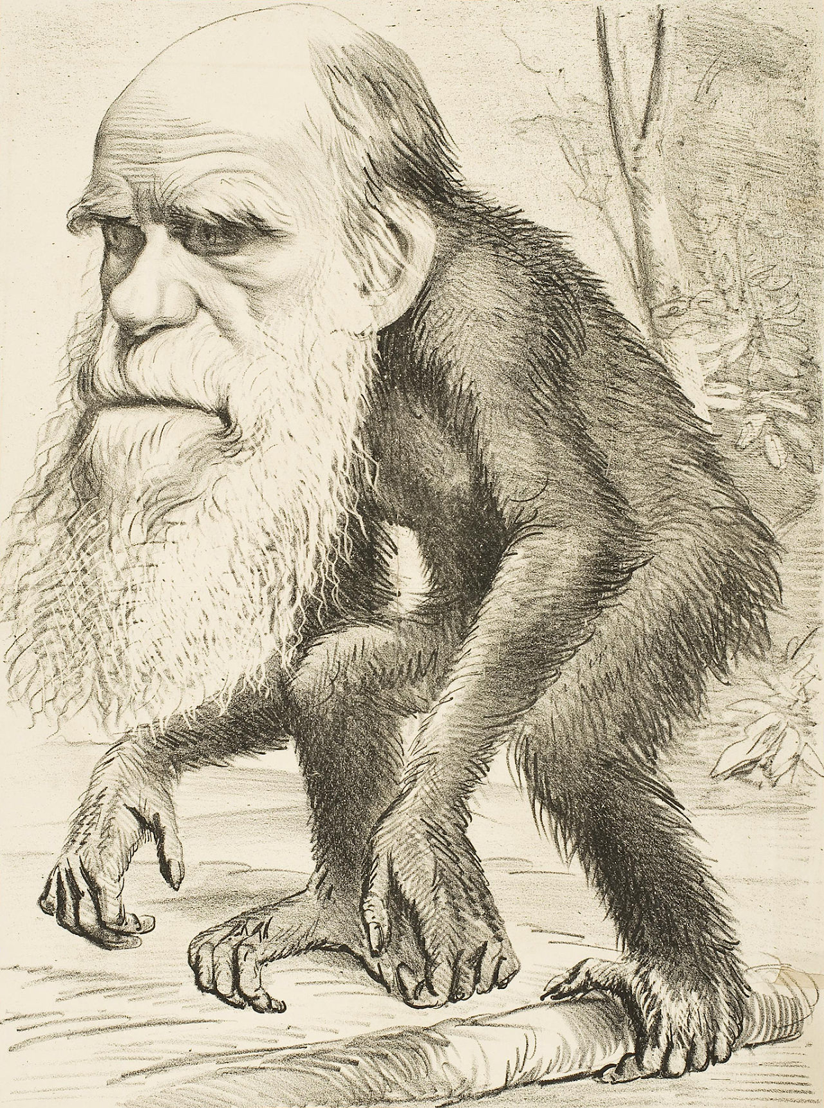
 If you start from scratch, it may take years to develop that intrinsic robustness.   

Being more wary of deleting old code is a cousin of this maxim:

 

 “Don't ever take a fence down until you know the reason it was put up” (Chesterton)

Let’s go to an Oryx and Crake style genetic engineering problem if you had the DNA 

skills to design creatures.   Should you improve on this ridiculous 

poorly designed creature (Photo:Samuel Blanc):

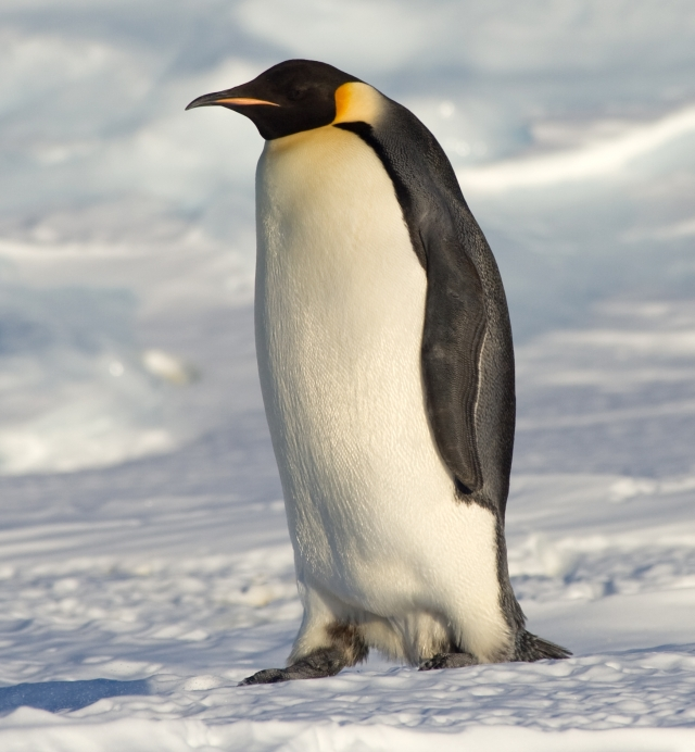
I mean it has wings but can’t fly?!   Some users may need that feature.  

 It swims but has feathers than can get wet?!   Why not make it like a dolphin.  

 Sure that creature might be better than version 1.0, but it might need many 

mods as it “dies” in various ways.

Another poorly designed creature that should be redesigned?   No brains and all spikes:

Make the brain bigger.  Make the legs longer.  Give it thumbs.

Having had a hedgehog as a pet, I am the first to admit they are ridiculous.  

But the hedgehog has needed little revision for 15 million years!

While the penguin and hedgehog are both very robust, if they traded continents both 

would probably die.   So sometimes the environment changes enough that starting from 

scratch is a good thing.   But never underestimate all the hidden talents in an 

evolved creature or piece of software!  Please read more about it in my new book:

Hello World for Smart Lights

 

I got three Philips Hue bulbs and a Philips Hue Bridge (basically a hub you need to attach to your router) and tried various Python interfaces to control them.  I found one I really like and here is a hello world:

 

 

(Yes, you could in theory run that program and control my bridge, but part of the Philips security is you need to be on the same network as the bridge)

Each bulb is set using HSB system that has (256^2, 256, 256) settings, and the program above cycles through the hues -- here are four stops along there:

 

I  found this to be quite fun and am thinking if I ever teach Intro Programming again I will base it on the Internet of Things-- the execution of commands becomes quite concrete!

Direct Light 3: what goes in the direct light function?

Part 1 of 3

Part 2 of 3

 

 In the previous two posts I discussed why one might want direct lighting as a separate computation.  But what goes in that function?

If we are just sampling a single light, then we need to bite the bullet and do a Monte Carlo integration with actual probability density functions.  These functions can either be defined over the area of the light, or the angles the light is seen through.  You can dive into all of that later-- it looks intimidating but is mainly like learning anything new with bad terminology and symbols-- just eat the pain :)

But for now, we can do it the easiest way possible and "just take my word for it".  After you have implemented this once, the written descriptions will make more sense.

First, pick a random point uniformly on the surface of the light.  Chapter 16 of this book will show you how to do this for various shapes.

The magic integral you need to solve, often referred to as the "rendering equation" is this:

 The key formula you evaluate is in red.  Area is the total area of the light.  The "rho" is the BRDF and for a diffuse (matte) surface that is "rho = reflectance / pi".   So pick a random point y uniformly on the light, see if x can "see" y by tracing a "shadow" ray from x to y (or vice-versa).  That's it!  It will be noisy for spherical lights (half the time, y is on the back and so will be shadowed, and the cosb will vary a lot), but it will work well for polygonal lights.  Worry about that later-- just get it to work.

What about multiple lights.  Three choices:

1. do one of these computations for each light and add them
2. pick one of the N lights at random, do the computation for that one light, and multiply by N
3. implement reservoir sampling like all the cool kids do (it is a new technique and works really well)

I endorse option 2 as your first step.  

 

Direct Light 2: integrating shadow rays into a path tracer

Part 1 of 3

Part 3 of 3

 

In my last post, I talked about using shadow rays to sample a light source directly.  Here is our old lovely but noisy path tracer:

vec3 ray_color(ray r)

  if (r hits an object)

       r = ray(hitpoint, generate a scattered  direction from the surface)

       return emitted(hitpoint) + reflectance*ray_color(r)

   else

        return background_color(r)

This works great provided the light emitting objects are big, but otherwise we get a lot of noise.  We also are crossing our fingers we don't get an infinite recursion.

Let's assume we have a magic function direct_light(vec3 p, reflectance_info ref).   Can we just do this to the return line above:

      return emitted(hitpoint) + direct(hitpont, ref_info) +reflectance*ray_color(r)

NOPE!  That would double count direct because that sacttered ray r might hit the light and get the emitted part.  So this is better:

     return direct(hitpont, ref_info) +reflectance*ray_color(r)

 BUT, if you see the light source in the picture, it will be black!  

And before we fix that, another problem is that if the surface is a perfect mirror, the direct lighting itself will be too noisy because only one point on the light matters.

So we need something like a "sees the light" flag on a ray.

vec3 ray_color(ray r)

   vec3 color = (0, 0, 0)

  if (r hits an object)

       if (r.should_see_lights)

            color +=  emitted(hitpoint)

            r = ray(hitpoint, generate a scattered  direction from the surface, should_r_see_lights_flag)

            if (r.should_see_light)

                    color += reflectance*ray_color(r)

            else

                    color += direct(hitpoint, ref_info) +reflectance*ray_color(r)

   else

        color += background_color(r)

  return color

Man that is pretty ugly!  But I don't know a much better way.  Be sure to set the viewing ray flags to "should_see_light = true".

 Are we done?  No.  For perfect mirrors, should_see_lights scattered rays should be set true.  For diffuse reflectors, false.  For glossy objects, it depends on the size of the light source.  Here, a lovely technique from Eric Veach is often used.   I would go with the "balance heuristic"-- it is easiest.  There is a wonderful figure from the paper that shows why this technique is needed:

 

So are we done?   No, there is one more issue.  Does the background "emit" light?  Isn't it a light source.  The answer is you can do it either way.  But if it is a light source, and you can hit it, we can get rid of the   if (r hits an object)  branch-- the background is always hit!  But if it has infinite radius where is the hitpoint?  I would say these design decisions are not obvious and I am on the fence even after trying all of them.

Next time: what goes in here: direct(hitpoint, ref_info)

 

 

 

     

What is direct lighting (next event estimation) in a ray tracer? Part 1 of 3

Part 2 of 3

Part 3 of 3

In Ray Tracing in One Weekend, we took a very brute force and we hope intuitive approach that didn't use "shadow rays", or as some on the whipper-snappers say "next event estimation".  Instead we scattered rays and they got "direct light" (light that is emitted by a radiant object, hits one surface, and is scattered to the camera) implicitly by having a ray randomly scatter and happen to hit to hit the light source.

Direct light with shadow rays can make some scenes much more efficient, and 99%+ of production ray tracers use shadow rays.  Let's look at a simple scene where the only thing in the world is two spheres, one diffusely reflective with reflectivity R, and one that absorbs all light but emits light uniformly in all directions, so it looks white.  So if we render just the light source, let's assume it is color RGB = (2,2,2).   (for now, assume RGB=(1,1,1) is white on the screen, and anything above (1,1,1) "burns out" to also be white-- this is a tone mapping issue which is its own field of study!  But we will just truncate above 1 for now which is the best tone mapping technique when measured by quality over effort :) ).

To color a pixel in the "brute force path tracer" paradigm, the color of an object is:

color = reflectivity * weighted_average(color coming into surface)

The weighted average says not all directions are created equal-- some influence the surface color more than others.  We can approximate that weighted average above by taking some random rays, weighting them, and averaging them:

for the six rays above, the weighted average is 

color = reflectivity*(w1*(0,0,0) + w2*(0,0,0) w3*(2,2,2) + w4*(2,2,2) w5*(0,0,0) + w6*(0,0,0))) / (w1+w2+w3+w4+w5+w6)

So reflectivity*(2/3, 2/3, 2.3) so a very light color.  If we had happened to have an extra ray randomly hit it would be reflectivity*(1,1,1) and if one more missed reflectivity*(1/3, 1/3, 1/3)

So we see why there is noise in ray tracings but also why the bottom of the sphere is black-- no scattered rays can hit the light. 

A key thing is this sort of Monte Carlo is any distribution of rays can be used, and any weighting functions can be used, and the picture will usually be "reasonable".  Surfaces attenuate light (with reflectivity-- their "color") and they preferentially average some directions over others.

Commonly, we will just make all the weights one, and make the ray directions "appropriate" for the surface type (like for a mirror, only one direction is chosen.  

The above is a perfectly reasonable way to compute shading from a light.   However, it gets very noisy for a small light (or more precisely, a light that subtends a small angle, light our biggest light, the Sun).

A completely different way to compute direct lighting is to view all those "missed" rays wasted, and only send rays that don't yield a zero contribution.  But to do that, we need to somehow figure out the weighting so that we get the same answer.

What we do there is just send rays toward the light source, and count the ones that hit (if they hit some other object, like a bird between the shaded sphere and the light, it's a zero).

So the rays are all random, but also only in directions toward the light.  Now the magic formula is

 color = MAGICCONSTANT*reflectivity*(w1*(0,0,0) + w2*(0,0,0) w3*(2,2,2) + w4*(2,2,2) w5*(0,0,0) + w6*(0,0,0))) / (w1+w2+w3+w4+w5+w6)

 What is different is:

1. what directions are chosen?

2. what are the weights?

3. What is the MAGICCONSTANT?     // will depend on the geometry for that specific point-- like it will have some distance squared attenuation in it

The place where we have freedom is 1.  Choose some way to sample directions toward the sphere.  For example, pick random points on the sphere and send rays to them.  Then 2 and 3 will be math.  The bad news is that the math is "advanced calculus" and looks intimidating because of the formulas and because 3D actually is confusing.  The good news is that that advanced calc can be done methodically.  More on that in a future post.

But great cheat!  Just use some common sense for guesses on 2 and 3 (checking the quality of your guesses with the more brute force technique) and your pictures will look pretty reasonable!  That is the beauty of weighted averages.

  

What is an "uber shader"?

 I am no expert on "uber shaders", but I am a fan.  These did not make much sense to me until recently.  First let's unpack the term a little bit.  The term "shader" in graphics has become almost meaningless.  To a first approximation it means "function".  So a "geometry shader" is a function that modifies geometry.  A "pixel shader" is a function that works on pixels.  In context those terms might mean something more specific.  

So "uber shader" is a general function?  No.

An uber shader is a very specific kind of function: it is one that evaluates a very particular BRDF, usually in the context of a particular rendering API.  The fact that it is a BRDF implies this is a "physically based" shader, so is ironically much more restricted than a general shader.  The "uber" refers to it being the "only material model you will ever need", and I think for most applications, that is true.  The one I have the most familiarity with (the only one I have implemented) is the Autodesk Standard Surface.

First let's get a little history.  Back in ancient times people would classify surfaces as "matte" or "shiny" and you would call a different function for each type of surface.  Every surface would somehow have a name or pointer or whatever to code to call about lighting or rays or whatever.  So they had different behavior.  Here is a typical example of some materials we used in our renderer three decades ago:

But sometime in the late 1990s some movie studios started making a single shader that encompassed all of these as well as some other effects such as retro-reflection and sheen and subsurface scattering.  (I don't know who came up with this idea first, but I think Sing-Choong Foo, one of the BRDF measurement and modeling pioneers that I overlapped with at Cornell, did one at PDI in the late 1990s... this may have been the first... please comment if you know anything about the hisotry which really ought to be documented).

Here is the Autodesk version's conceptual graph of how the shader is composed:

So a bunch of different shaders are added in linear combinations, and the weights may be constant or may be functions.  This is a bit daunting looking.  Let's show how you would make a metal (like copper!):  First set opacity=1, coat=0, metalness=1.   This causes most of the graph to be irrelevant:

Now let's do a diffuse surface.  Opacity=1, coat = 0, metalness=0, specular=0,transmission=0,sheen=0,subsurface=0.  Phew!  Again most of the graph drops away:

So why has this, for the most part, won out over categorical shaders that are different?  Having implemented the above shader along with my colleague and friend Bob Alfieri, I really like it for streamlining software.  Here is your shader black box!   Further, you can point to the external document and get data in that format.  

But I suspect that is not the only reason uber shaders have taken over.  Note that we could have set metalness=0.5 above.  So this thing is half copper metal and half pink diffuse.  Does that make any sense as a physical material?  Probably not.  And isn't the whole point of a BRDF to restrict us to physical materials?  I think such unphysical combinations serve two purposes:

1. Artistic expression.  We usually do physically-based BRDF as a guide to keeping things plausible and robust.  But an artistic production like a game or movie might look better with nonphysical combinations, so why not expose the knobs!
2. LOD and antialiasing. A pixel or region of an object may cover more than one material.  So the final pixel color should account for both BRDF.  Combining them in the shading calculation allows sparser sampling.

Finally, graphics needs to be fast both in development and production.  So the compiler ecosystem is here.  I don't know so much about that, which is a credit to the compiler/language people who do :)

.

A call to brute force

 In the writing of the new edition of Marschner's and my graphics text, we tried to add more "basics" on light and material interaction (I don't mean BRDF stuff-- I mean more dielectrics) and more on brute force simulation of light transport.  In the "how would you maximally brute force a ray tracer) we wrote this:

 

Basically, it's just a path tracer run with *only* smooth dielectrics and Beer's Law.  If you model a scene with all the microgeometry and allow some of it to absorb, you can get colored paint with a rough surface.  Here is an few  figures from my thesis (and it was an old idea then!):

Doing the brute force path tracing is slow and dealing with the micro-particles is slow, so we invent BRDFs and other bulk properties, but that is all for efficiency.  When we wrote this, which is a classic treatment people use in the classroom all the time, we were thinking it was just for education and  for reference solutions (like Eugene d'Eon has done for skin for example), but since Monte Carlo path tracing is almost infinitely parallel, why not do this on a huge crowd sourced network of computers (in the spirit folding@home)?

I am thinking for images of ordinary things whose microgeometry would be easy to model.  For example a lamp shade with a white lining:

Another example of something very complex visually that might be modeled procedurally (https://iswallquality.blogspot.com/2016/07/fresh-snow-close-up-wallpaper-hd.html):

 

Or a glass of beer or... (on and on).

So what would be needed:

1. some base path tracer with a procedural model we could all install and run
2. some centralized job coordination server that doled out random seeds and combined results 
3. an army of nerds willing to do this with idle cycles rather than coin mining

I don't have the systems chops to know how to best do this.  Anyone?   I will take the discussion to twitter!