In a physically-based renderer, your RGB values are not confined to [0,1] and your need to deal with that somehow.
The simplest thing is to clamp them to zero to one. In my own C++ code:
inline vec3 vec3::clamp() {
if (e[0] < real(0)) e[0] = 0;
if (e[1] < real(0)) e[1] = 0;
if (e[2] < real(0)) e[2] = 0;
if (e[0] > real(1)) e[0] = 1;
if (e[1] > real(1)) e[1] = 1;
if (e[2] > real(1)) e[2] = 1;
return *this;
}
A more pleasing result can probably be had by applying a "tone mapping" algorithm. The easiest is probably Eric Reinhard's "L/(1+L)" operator from the Equation 3 of this paper
Here is my implementation of it. You still need to clamp because of highly saturated colors, and purists wont like my luminance formula (1/3.1/3.1/3) but never listen to purists :)
void reinhard_tone_map(real mid_grey = real(0.2)) {
// using even values for luminance. This is more robust than standard NTSC luminance
// Reinhard tone mapper is to first map a value that we want to be "mid gray" to 0.2// And then we apply the L = 1/(1+L) formula that controls the values above 1.0 in a graceful manner.
real scale = (real(0.2)/mid_grey);
for (int i = 0; i < nx*ny; i++) {
vec3 temp = scale*vdata[i];
real L = real(1.0/3.0)*(temp[0] + temp[1] + temp[2]);
real multiplier = ONE/(ONE + L);
temp *= multiplier;
temp.clamp();
vdata[i] = temp;
}
}
This will slightly darken the dark pixels and greatly darken the bright pixels. Equation 4 in the Reinhard paper will give you more control. The cool kids have been using "filmic tone mapping" and it is the best tone mapping I have seen, but I have not implemented it (see title to this blog post)
Sunday, February 17, 2019
Thursday, February 14, 2019
Picking points on the hemisphere with a cosine density
NOTE: this post has three basic problems. It assumes property 1 and 2 are true, and there is a missing piece at the end that keeps us from showing anything :)
This post results from a bunch of conversations with Dave Hart and the twitter hive brain. There are several ways to generate a random Lambertian direction from a point with surface normal N. One way is inspired by a cool paper by Sbert and Sandez where he simultaniously generated many form factors by repeatedly selecting a uniformly random 3D line in the scene. This can be used to generate a direction with a cosine density, an idea first described, as far as I know, by Edd Biddulph.
I am going to describe it here using three properties, each of which I don't have a concise proof for. Any help appreciated! (I have algebraic proofs-- they just aren't enlightening--- hoping for a clever geometric observation).
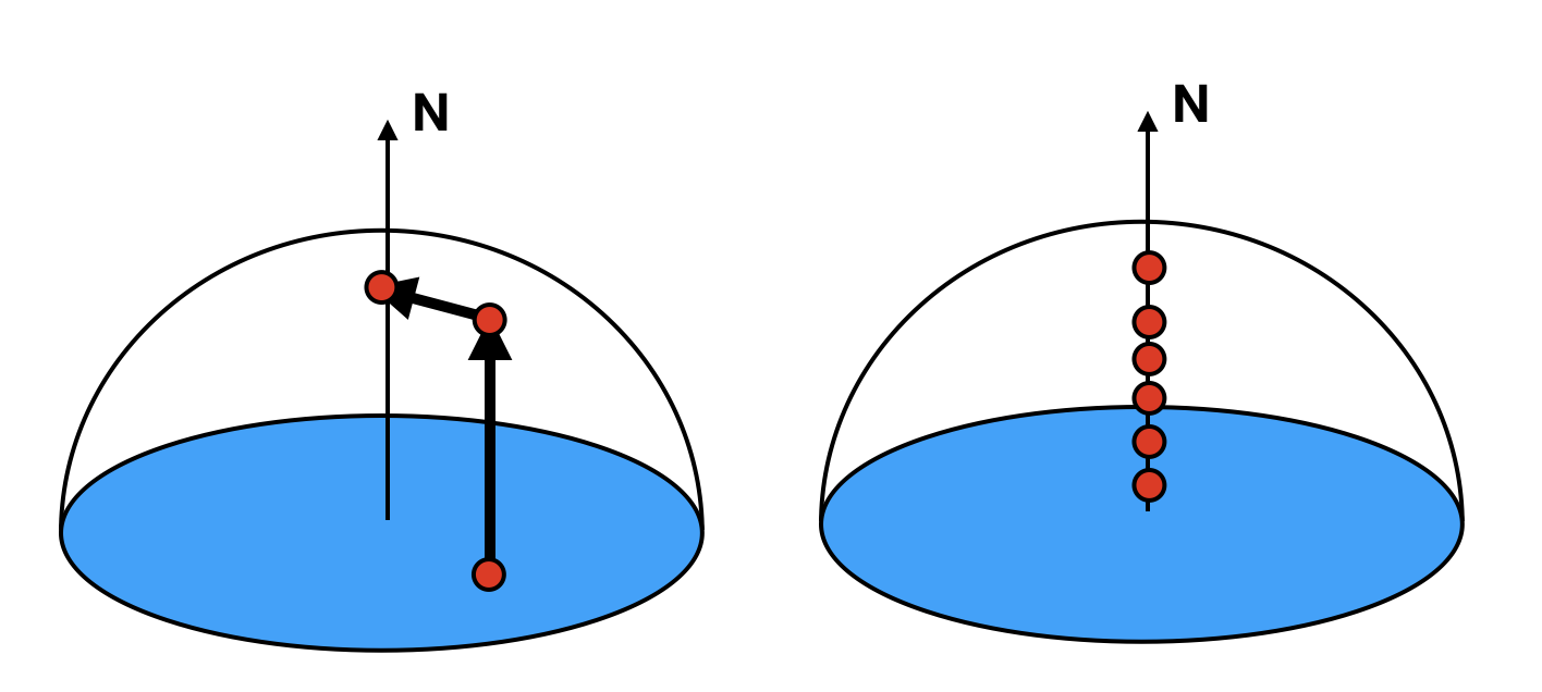
Property 1: Nusselt Analog: uniform random points on an equatorial disk projected onto the sphere have a cosine density. So in the figure, the red points, if all of them projected, have a cosine density.

Property 2: (THIS PROPERTY IS NOT TRUE-- SEE COMMENTS) The red points in the diagram above when projected onto the normal, will have a uniform density along it:

Now if we accept Property 3, we can first generate a random point on a sphere by first choosing a random phi uniformly theta = 2*PI*urandom(), and then choose a random height from negative 1 to 1, height = -1 + 2*urandom()
In XYZ coordinates we can convert this to:
z = -1 + 2*urandom()
phi = 2*PI*urandom()
x = cos(phi)*sqrt(1-z*z)
y = sin(phi)*sqrt(1-z^2)
Similarly from property 2 we can given a random point (x,y) on a unit disk in the XY plane, we can generate a direction with cosine density when N = the z axis:
(x,y) = random on disk
z = sqrt(1-x*x-y*y)
To generate a cosine direction relative to a surface normal N, people usually construct a local basis, ANY local basis, with tangent and bitangent vectors B and T and change coordinate frames:
get_tangents(B,T,N)
(x,y) = random on disk
z = sqrt(1-x*x-y*y)
direction = x*B + y*T + z*N
There is finally a compact and robust way to write get_tangents. So use that, and your code is fast and good.
But can we do this show that using a uniform random sphere lets us do this without tangents?
So we do this:
P = (x,y,z) = random_on_unit_sphere
D = unit_vector(N + P)
So D is the green dot while (N+P) is the red dot:

So is there a clever observation that the green dot is either 1) uniform along N, or 2, uniform on the disk when projected?
Tuesday, February 12, 2019
Adding point and directional lights to a physically based renderer
Suppose you have a physically based renderer with area lights. Along comes a model with point and directional lights. Perhaps the easiest way to deal with them is convert them to a very small spherical light source. But how do you do that in a way that gets the color right? IF you have things set up so they tend to be tone mapped (a potential big no in physically-based renderer), meaning that a color of (1,1,1) will be white, and (0.2,0.2,0.2) a mid-grey (gamma-- so not 0.5-- the eye does not see intensities linearly), then it is not so bad.
Assume you have a spherical light with radius R at position C and emitted radiance (E,E,E). When it is straight up from a white surface (so the sun at noon at the equator), you get this equation (about) for the color at a point P
reflected_color = (E,E,E)*solid_angle_of_light / PI
The solid angle of the light is its projected area on the unit sphere around the illuminated point, or approximately:
solid_angle_of_light = PI*R^2 /distance_squared(P,C)
So
reflected_color = (E,E,E)*(R / distance(P,C))^2
If we want the white surface to be exactly white then
E = (distance(P,C) / R)^2
So pick a small R (say 0.001), pick a point in your scene (say the one the viewer is looking at, or 0,0,0), and and set E as in the green equation
Suppose the RGB "color" given for the point source is (cr, cg, cb). Then just multiply the (E,E,E) by those components.
Directional lights are a similar hack, but a little less prone to problems of whther falloff was intended. A directional light is usually the sun, and it's very far away. Assume the direction is D = (dx,dy,dz)
Pick a big distance (one that wont break your renderer) and place the center in that direction:
C = big_constant*D
Pick a small radius. Again one that wont break your renderer. Then use the green equation above.
Now sometimes the directional sources are just the Sun and will look better if you give them the same angular size for the Sun. If your model is in meters, then just use distance = 150,000,000,000m. OK now your program will break due to floating point. Instead pick a somewhat big distance and use the right ratio of Sun radius to distance:
R = distance *(695,700km / 149,597,870km)
And your shadows will look ok
Subscribe to:
Posts (Atom)